Examples
The example data files can be downloaded from the github project page
DNS case
This velocity field is from a DNS simulation of an Homogeneous Isotropic Turbulence (HIT) case.
Using default input file example_dataHIT.nc, default scheme least square filter and default detection swirling strength we test here two cases:
- Case 1: threshold on swirling strength = 0.0
- Case 2: threshold on swirling strength = 0.1
- Case 3: threshold on swirling strength = 0.2
- Case 4: threshold on swirling strength = 0.4
If you set self.normalization_flag = True on the classes.py module, the value of swirling strength will be normalized. The values of the threshold must be set to avoid unnecessary noise.


Case 4
$ vortexfitting -t 0.4 -i data/example_dataHIT.nc

9 vortices detected with 8 accepted.
Below two vortices are displayed, where in the left we have the normal field and to the right we have the advection velocity subtracted.


| Case | Threshold | Detected | Accepted |
|---|---|---|---|
| 1 | 0.0 | 361 | 84 |
| 2 | 0.1 | 162 | 72 |
| 3 | 0.2 | 58 | 40 |
| 4 | 0.4 | 9 | 8 |
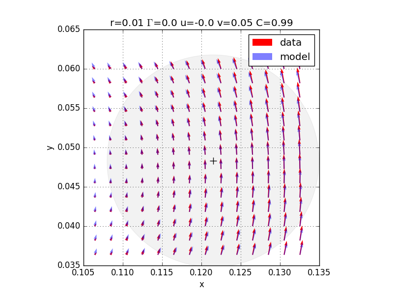
PIV case - NetCDF file
For PIV data we need to update the format, to match NetCDF file.
It is done with the -ft piv_netcdf (file type) argument.
Here, since we have an advection velocity, we have to set self.normalization_flag = True and self.normalization_direction = ‘y’. This is done directly in the classes.py module.
The -rmax argument leaves the software calculate the initial radius.
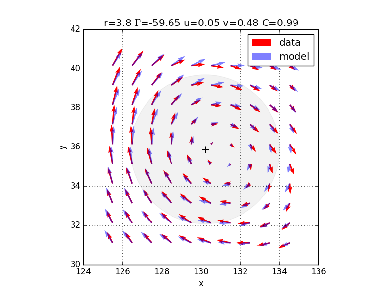
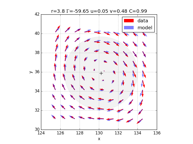
$ vortexfitting -i data/example_dataPIV.nc -ft piv_netcdf -t 1.5 -rmax 0

203 vortices detected with 24 accepted.
Below two vortices are displayed, where in the left we have the normal field and to the right we have the advection velocity subtracted.


PIV case - Tecplot file
For PIV data with Tecplot, we need to update the format, to match Tecplot file.
It is done with the -ft piv_tecplot (file type) argument.
$ vortexfitting.py data/adim_vel_{:06d}.dat -first 10 -t 5 -b 10 -ft piv_tecplot

An average field can be subtracted, using -mf argument (mean file)
If you want to analyze a set of images, use arguments -first, -last and -step.
(please modify data input to format the image number: dim_vel_{:06d}.dat with -first 10 is formatted as dim_vel_000010.dat).
$ vortexfitting.py -i data/dim_vel_{:06d}.dat -mf data/mean.dat -t 50 -first 10 -ft piv_tecplot
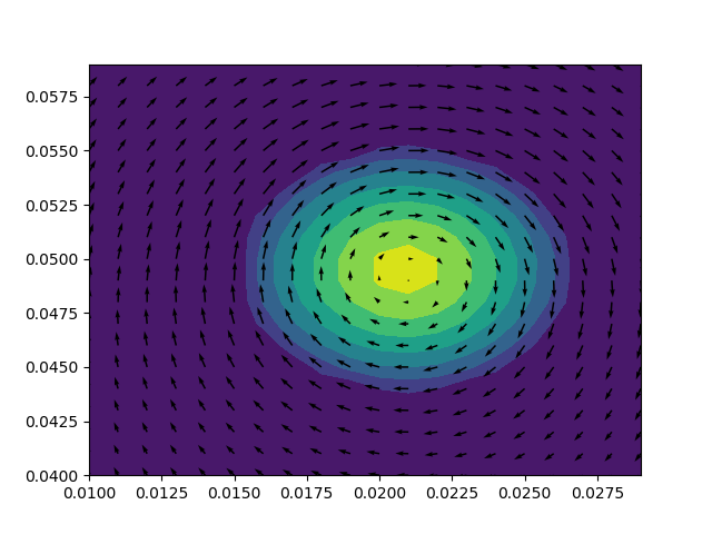
As presented in the image, one main vortex is found in the velocity field provided.
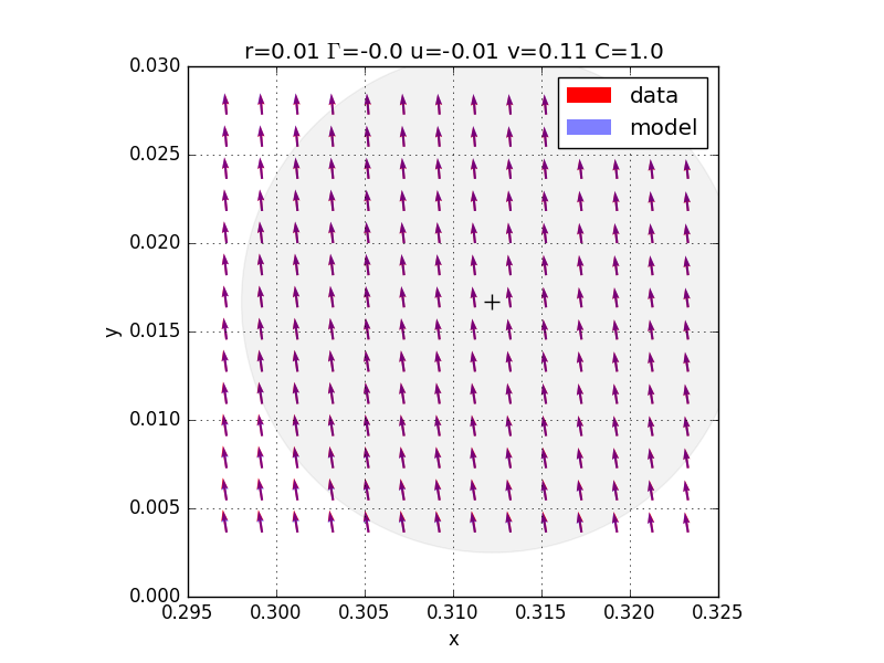
Numerical case - OpenFOAM file
A columnar Lamb-Oseen vortex is generated on OpenFOAM. By default, data are extracted in a text file, with a .raw extension.
Here, a z-plane is extracted, with a 100x100 mesh.  data are exported.
The spatial mesh for this simulation is quite small, so the default initial radius (rmax = 10) is too large.
Specify a smaller value (close to the spatial mesh); -rmax 0 gets an initial radius of 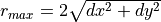 ,
,
with  and
and  the spatial resolution.
$ vortexfitting.py -i data/example_Ub_planeZ_0.01.raw -ft openfoam -rmax 0.0